Please visit this page for a code implementation of the fixed step size gradiant method and this page for a code implementation of the steepest gradiant method.
Suppose that we are given a point x(k). To find the next point x(k+1), we start at x(k) and move by an amount −αk∇f(x(k)), where αk is a positive scalar called the step size. This procedure leads to the following iterative algorithm:
x(k+1)=x(k)−αk∇f(x(k)).
We refer to this as a gradient descent algorithm (or simply a gradient algorithm).
The method of steepest descent is a gradient algorithm where the step size αk is chosen to achieve the maximum amount of decrease of the objective function at each individual step. Specifically, αk is chosen to minimize ϕk(α)≜f(x(k)−α∇f(x(k))). In other words,
αk=α≥0argminf(x(k)−α∇f(x(k))).
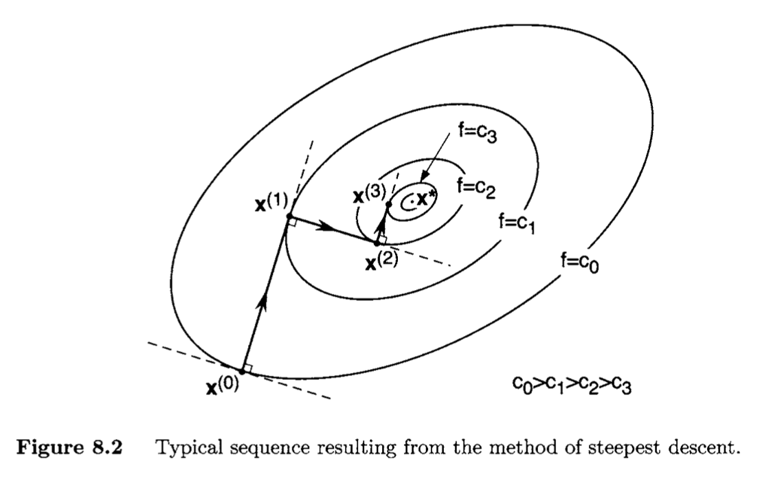
Observe that the method of steepest descent moves in orthogonal steps, as stated in the following proposition.
If {x(k)}k=0∞ is a steepest descent sequence for a given function f:Rn→R, then for each k the vector x(k+1)−x(k) is orthogonal to the vector x(k+2)−x(k+1).
which completes the proof.
The proposition above implies that ∇f(x(k)) is parallel to the tangent plane to the level set {f(x)=f(x(k+1))} at x(k+1). Note that as each new point is generated by the steepest descent algorithm, the corresponding value of the function f decreases in value, as stated below.
Let us now see what the method of steepest descent does with a quadratic function of the form
f(x)=21x⊤Qx−b⊤x,
where Q∈Rn×n is a symmetric positive definite matrix, b∈Rn, and x∈Rn. The unique minimizer of f can be found by setting the gradient of f to zero, where
∇f(x)=Qx−b,
because D(x⊤Qx)=x⊤(Q+Q⊤)=2x⊤Q, and D(b⊤x)=b⊤. There is no loss of generality in assuming Q to be a symmetric matrix. For if we are given a quadratic form x⊤Ax and A=A⊤, then because the transposition of a scalar equals itself, we obtain
(x⊤Ax)⊤=x⊤A⊤x=x⊤Ax.
Hence,
x⊤Ax=21x⊤Ax+21x⊤A⊤x=21x⊤(A+A⊤)x≜21x⊤Qx.
Note that
(A+A⊤)⊤=Q⊤=A+A⊤=Q.
The Hessian of f is F(x)=Q=Q⊤>0. To simplify the notation we write g(k)=∇f(x(k)). Then, the steepest descent algorithm for the quadratic function can be represented as
In the quadratic case, we can find an explicit formula for αk. We proceed as follows. Assume that g(k)=0, for if g(k)=0, then x(k)=x∗ and the algorithm stops. Because αk≥0 is a minimizer of ϕk(α)=f(x(k)−αg(k)), we apply the FONC to ϕk(α) to obtain
ϕk′(α)=(x(k)−αg(k))⊤Q(−g(k))−b⊤(−g(k)).
Therefore, ϕk′(α)=0 if αg(k)⊤Qg(k)=(x(k)⊤Q−b⊤)g(k). But
x(k)⊤Q−b⊤=g(k)⊤.
Hence,
αk=g(k)⊤Qg(k)g(k)⊤g(k).
In summary, the method of steepest descent for the quadratic takes the form
We can investigate important convergence characteristics of a gradient method by applying the method to quadratic problems. The convergence anaylysis is more convenient if instead of working with f we deal with
V(x)=f(x)+21x∗⊤Qx∗=21(x−x∗)⊤Q(x−x∗),
where Q=Q⊤>0. The solution point x∗ is obtained by solving Qx=b; that is, x∗=Q−1b. The function V differs from f only by a constant 21x∗⊤Qx∗. We begin our analysis with the following useful lemma that applies to a general gradient algorithm.
The proof is by direct computation. Note that if g(k)=0, then the desired result holds trivially. In the remainder of the proof, assume that g(k)=0. We first evaluate the expression
V(x(k))V(x(k))−V(x(k+1))
To facilitate computations, let y(k)=x(k)−x∗. Then, V(x(k))=21y(k)⊤Qy(k). Hence,
Note that γk≤1 for all k, because γk=1−V(x(k+1))/V(x(k)) and V is a nonnegative function. If γk=1 for some k, then V(x(k+1))=0, which is equivalent to x(k+1)=x∗. In this case we also have that for all i≥k+1, x(i)=x∗ and γi=1. It turns out that γk=1 if and only if either gˉ(k)=0 or g(k) is an eigenvector of Q (see Lemma 3).
We are now ready to state and prove our key convergence theorem for gradient methods. The theorem gives a necessary and sufficient condition for the sequence {x(k)} generated by a gradient method to converge to x∗; that is, x(k)→x∗ or limk→∞x(k)=x∗.
Let {x(k)} be the sequence resulting from a gradient algorithm x(k+1)=x(k)−αkg(k). Let γk be as defined in Lemma 1, and suppose that γk>0 for all k. Then, {x(k)} converges to x∗ for any initial condition x(0) if and only if
From Lemma 1 we have V(x(k+1))=(1−γk)V(x(k)), from which we obtain
V(x(k))=(i=0∏k−1(1−γi))V(x(0))
Assume that γk<1 for all k, for otherwise the result holds trivially. Note that x(k)→x∗ if and only if V(x(k))→0. By the equation above we see that this occurs if and only if ∏i=0∞(1−γi)=0, which, in turn, holds if and only if ∑i=0∞−log(1−γi)=∞ (we get this simply by taking logs). Note that by Lemma 1, 1−γi≥0 and log(1−γi) is well-defined [log(0) is taken to be −∞]. Therefore, it remains to show that ∑i=0∞−log(1−γi)=∞ if and only if
i=0∑∞γi=∞
We first show that ∑i=0∞γi=∞ implies that ∑i=0∞−log(1−γi)=∞. For this, first observe that for any x∈R,x>0, we have log(x)≤x−1
[this is easy to see simply by plotting log(x) and x−1 versus x ]. Therefore, log(1−γi)≤1−γi−1=−γi, and hence −log(1−γi)≥γi. Thus, if ∑i=0∞γi=∞, then clearly ∑i=0∞−log(1−γi)=∞.
Finally, we show that ∑i=0∞−log(1−γi)=∞ implies that ∑i=0∞γi=∞. We proceed by contraposition. Suppose that ∑i=0∞γi<∞. Then, it must be that γi→0. Now observe that for x∈R,x≤1 and x sufficiently close to 1 , we have log(x)≥2(x−1) [as before, this is easy to see simply by plotting log(x) and 2(x−1) versus x]. Therefore, for sufficiently large i, log(1−γi)≥2(1−γi−1)=−2γi, which implies that −log(1−γi)≤2γi. Hence, ∑i=0∞γi<∞ implies that ∑i=0∞−log(1−γi)<∞.
This completes the proof.
If g(k)=0 for some k, then x(k)=x∗ and the result holds. So assume that g(k)=0 for all k. Recall that for the steepest descent algorithm,
αk=g(k)⊤Qg(k)g(k)⊤g(k).
Substituting this expression for αk in the formula for γk yields
γk=(g(k)⊤Qg(k))(g(k)⊤Q−1g(k))(g(k)⊤g(k))2.
Note that in this case γk>0 for all k. Furthermore, by Lemma 8.2, we have γk≥(λmin(Q)/λmax(Q))>0. Therefore, we have ∑k=0∞γk=∞, and hence by Theorem 8.1 we conclude that x(k)→x∗.
Consider now a gradient method with fixed step size; that is, αk=α∈R for all k. The resulting algorithm is of the form
x(k+1)=x(k)−αg(k).
We refer to the algorithm above as a fixed-step-size gradient algorithm. The algorithm is of practical interest because of its simplicity. In particular, the algorithm does not require a line search at each step to determine αk, because the same step size α is used at each step. Clearly, the convergence of the algorithm depends on the choice of α, and we would not expect the algorithm to work for arbitrary α. The following theorem gives a necessary and sufficient condition on α for convergence of the algorithm.
Therefore, substituting the above into the formula for γk, we get
γk≥α(λmin(Q))2(λmax(Q)2−α)>0.
Therefore, γk>0 for all k, and ∑k=0∞γk=∞. Hence, by Theorem 8.1 we conclude that x(k)→x∗.
⇒ : We use contraposition. Suppose that either α≤0 or α≥2/λmax(Q).
Let x(0) be chosen such that x(0)−x∗ is an eigenvector of Q corresponding to the eigenvalue λmax(Q). Because
We now turn our attention to the issue of convergence rates of gradient algorithms. In particular, we focus on the steepest descent algorithm. We first present the following theorem.
In the proof of Theorem 2, we showed that γk≥λmin(Q)/λmax(Q). Therefore,
V(x(k))V(x(k))−V(x(k+1))=γk≥λmax(Q)λmin(Q)
and the result follows.
Theorem 4 is relevant to our consideration of the convergence rate of the steepest descent algorithm as follows. Let
r=λmin(Q)λmax(Q)=∥Q∥∥∥Q−1∥∥,
called the condition number of Q. Then, it follows from Theorem 8.4 that
V(x(k+1))≤(1−r1)V(x(k)).
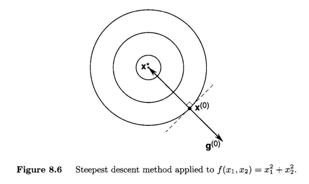
The term (1−1/r) plays an important role in the convergence of {V(x(k))} to 0 (and hence of {x(k)} to x∗). We refer to (1−1/r) as the convergence ratio. Specifically, we see that the smaller the value of (1−1/r), the smaller V(x(k+1)) will be relative to V(x(k)), and hence the "faster" V(x(k)) converges to 0 , as indicated by the inequality above. The convergence ratio (1−1/r) decreases as r decreases. If r=1, then λmax(Q)=λmin(Q), corresponding to circular contours of f (see Figure 8.6). In this case the algorithm converges in a single step to the minimizer. As r increases, the speed of convergence of {V(x(k))} (and hence of {x(k)} ) decreases. The increase in r reflects that fact that the contours of f are more eccentric (see, e.g., Figure 8.7). We refer the reader to [88, pp. 238, 239] for an alternative approach to the analysis above.
To investigate the convergence properties of {x(k)} further, we need the following definition.
Given a sequence {x(k)} that converges to x∗, that is, limk→∞∥∥x(k)−x∗∥∥=0, we say that the order of convergence is p, where p∈R, if
0<k→∞lim∥∥x(k)−x∗∥∥p∥∥x(k+1)−x∗∥∥<∞.
If for all p>0
k→∞lim∥∥x(k)−x∗∥∥p∥∥x(k+1)−x∗∥∥=0,
then we say that the order of convergence is ∞.
Note that in the definition above, 0/0 should be understood to be 0 .
The order of convergence of a sequence is a measure of its rate of convergence; the higher the order, the faster the rate of convergence. The order of convergence is sometimes also called the rate of convergence (see, e.g., [96]). If p=1 (first-order convergence) and limk→∞∥∥x(k+1)−x∗∥∥/∥∥x(k)−x∗∥∥=1, we say that the convergence is sublinear. If p=1 and limk→∞∥x(k+1)−x∗∥/∥x(k)−x∗∥<1, we say that the convergence is linear. If p>1, we say that the convergence is superlinear. If p=2 (second-order convergence), we say that the convergence is quadratic.